Normal Distribution - Advanced Probability Calculation Using a z Table
The Empirical Rule is useful for finding simple probabilities for a distribution, but it is necessary to use a table of values to find more specific probabilities. If we use the example of IQ scores, with a mean of 100 and a standard deviation of 15, we have previously seen that the probability, for example, that a randomly-selected individual scores between 100 and 115 is about 34%, or .34. But what if we wanted to know the probability that a student scores between, say, 105 and 118? The Empirical Rule is insufficient for determining this probability.
A special curve called the Standard Normal Curve (SNC) must be used for finding probabilities not covered by the Empirical Rule. The SNC has been standardized to have a mean of 0 and a standard deviation of 1. Additionally, we use the term "z-value" to designate a particular location on the SNC. Here is a sketch of the SNC:
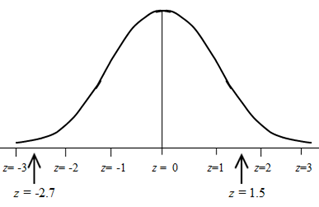
Notice that z-values do not have to be whole number values. The sketch shows both whole-number values for z and some with decimal values.
Before we can calculate probabilities for particular IQ scores, we need to be able to determine probabilities on the SNC, using z-values. We can do this with the help of a table of z-values. Later, we will be able to calculate probabilities for IQ scores or for many other real-world examples.
Let's first get familiar with the table of z-values, which is found in every Statistics text and on the internet. Here is a portion of a z-table:
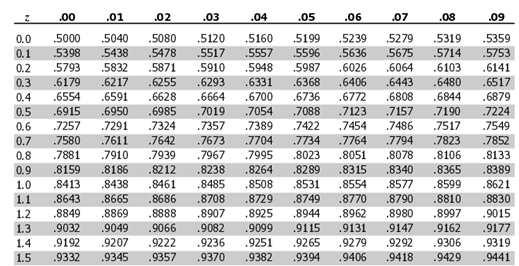
You will see that the z-values are listed in the leftmost column. They are correct to one decimal place. Let's use the chart to determine a particular probability.
What is the probability that a z value is less than or equal to 1.5? This would be written more formally as: P(z ≤ 1.5). The first step is to draw a sketch and to locate the approximate location of z = 1.5.
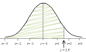
The sketch shows the approximate location of the z-value of 1.5. We want to determine the probability that a z-value is less than or equal to 1.5, so we shade the region of the SNC to the left of z = 1.5, as shown. This is where the z-table is used. We find the z-value of 1.5 in the first column, and directly to its right is the value .9332. This tells us that the probability that a z value is less than or equal to 1.5 is about .9332. Thus, the shaded region is about 93.32% of the entire curve.
Let's try another example. This time, determine the probability that a z-value is less than or equal 1.12, and this is written as P(z ≤ 1.12).
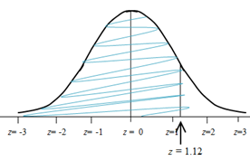
We make a sketch and shade the region to the left and look for a z value of 1.12 in the first column, but we can't find it. The nearest value is a z value of 1.1. The first column only lists z-values to one decimal place, and the number 1.12 has two decimal places. We look at the very top row of the chart, and we use the column headed by ".02" because this is where we find that second decimal place of the z value of 1.12. We now go down the .02 column until we intersect with the 1.1 row, and we are now at the probability for a z value of 1.12. The probability is .8686. Thus, the shaded region is about 86.86% of the entire curve, and the probability that a z value is less than or equal to 1.12 is .8686.
Notice that in both of these examples, we determined the probability that a z value was less than or equal to a particular value. The table gave us those probabilities directly. But what if, in the preceding example, we had been asked the probability that the z value was greater than 1.12? We could easily calculate this probability by noting that the entire area under the curve is 100%, or 1. Thus, to calculate the probability that a z value is greater than 1.12, we find the probability in the table for 1.12, as we did earlier, but now we subtract that probability from 1. Thus, the probability that z is greater than 1.12 is: 1 - .8686 = .1314.
The final calculation that is necessary for successfully using a z table is the determination of the probability that a z value is between two values. For example, to find the probability that a z value is between 1.12 and 1.5, we would first draw a sketch and shade the region between the two z values, as shown.
We must use the table, but this time we look up both z values and find the probability associated with each. For z = 1.5, we already found that the entire probability to its left is .9332. For z = 1.12, we already found that the entire probability to its left is .8686.
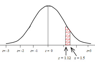
In order to find the probability that a z value is between 1.12 and 1.15, we determine the difference of the two probabilities.
Thus, to calculate the probability that a z value is between 1.12 and 1.5, we find the difference: .9332 - .8686 = .0646. We now know that about 6.46% of the entire bell curve is between z = 1.12 and 1.5.
You can find the entire z table, which will include negative values of z, in your Statistics book or on the internet. We used only a portion of the entire table for these examples. The procedures for determining probabilities with negative values of z are identical.
A special curve called the Standard Normal Curve (SNC) must be used for finding probabilities not covered by the Empirical Rule. The SNC has been standardized to have a mean of 0 and a standard deviation of 1. Additionally, we use the term "z-value" to designate a particular location on the SNC. Here is a sketch of the SNC:
Notice that z-values do not have to be whole number values. The sketch shows both whole-number values for z and some with decimal values.
Before we can calculate probabilities for particular IQ scores, we need to be able to determine probabilities on the SNC, using z-values. We can do this with the help of a table of z-values. Later, we will be able to calculate probabilities for IQ scores or for many other real-world examples.
Let's first get familiar with the table of z-values, which is found in every Statistics text and on the internet. Here is a portion of a z-table:
You will see that the z-values are listed in the leftmost column. They are correct to one decimal place. Let's use the chart to determine a particular probability.
What is the probability that a z value is less than or equal to 1.5? This would be written more formally as: P(z ≤ 1.5). The first step is to draw a sketch and to locate the approximate location of z = 1.5.
The sketch shows the approximate location of the z-value of 1.5. We want to determine the probability that a z-value is less than or equal to 1.5, so we shade the region of the SNC to the left of z = 1.5, as shown. This is where the z-table is used. We find the z-value of 1.5 in the first column, and directly to its right is the value .9332. This tells us that the probability that a z value is less than or equal to 1.5 is about .9332. Thus, the shaded region is about 93.32% of the entire curve.
Let's try another example. This time, determine the probability that a z-value is less than or equal 1.12, and this is written as P(z ≤ 1.12).
We make a sketch and shade the region to the left and look for a z value of 1.12 in the first column, but we can't find it. The nearest value is a z value of 1.1. The first column only lists z-values to one decimal place, and the number 1.12 has two decimal places. We look at the very top row of the chart, and we use the column headed by ".02" because this is where we find that second decimal place of the z value of 1.12. We now go down the .02 column until we intersect with the 1.1 row, and we are now at the probability for a z value of 1.12. The probability is .8686. Thus, the shaded region is about 86.86% of the entire curve, and the probability that a z value is less than or equal to 1.12 is .8686.
Notice that in both of these examples, we determined the probability that a z value was less than or equal to a particular value. The table gave us those probabilities directly. But what if, in the preceding example, we had been asked the probability that the z value was greater than 1.12? We could easily calculate this probability by noting that the entire area under the curve is 100%, or 1. Thus, to calculate the probability that a z value is greater than 1.12, we find the probability in the table for 1.12, as we did earlier, but now we subtract that probability from 1. Thus, the probability that z is greater than 1.12 is: 1 - .8686 = .1314.
The final calculation that is necessary for successfully using a z table is the determination of the probability that a z value is between two values. For example, to find the probability that a z value is between 1.12 and 1.5, we would first draw a sketch and shade the region between the two z values, as shown.
We must use the table, but this time we look up both z values and find the probability associated with each. For z = 1.5, we already found that the entire probability to its left is .9332. For z = 1.12, we already found that the entire probability to its left is .8686.
In order to find the probability that a z value is between 1.12 and 1.15, we determine the difference of the two probabilities.
Thus, to calculate the probability that a z value is between 1.12 and 1.5, we find the difference: .9332 - .8686 = .0646. We now know that about 6.46% of the entire bell curve is between z = 1.12 and 1.5.
You can find the entire z table, which will include negative values of z, in your Statistics book or on the internet. We used only a portion of the entire table for these examples. The procedures for determining probabilities with negative values of z are identical.
|
Related Links: Math Probability and Statistics Normal Distribution - Real-World Problems Using z Values Scatterplot |
To link to this Normal Distribution - Advanced Probability Calculation Using a z Table page, copy the following code to your site: